Using Pysketcher to Create Principal Sketches of Physics Problems

Author:Hans Petter Langtangen Date:Apr 1, 2012

Abstract. Pysketcher is a Python package which allows principal sketches of physics and mechanics problems to be realized through short programs instead of interactive (and potentially tedious and inaccurate) drawing. Elements of the sketch, such as lines, circles, angles, forces, coordinate systems, etc., are realized as objects and collected in hierarchical structures. Parts of the hierarchical structures can easily change line styles and colors, or be copied, scaled, translated, and rotated. These features make it straightforward to move parts of the sketch to create animation, usually in accordance with the physics of the underlying problem. Exact dimensioning of the elements in the sketch is trivial to obtain since distances are specified in computer code.

Pysketcher is easy to learn from a number of examples. Beyond essential Python programming and a knowledge about mechanics problems, no further background is required.

A First Glimpse of Pysketcher

Formulation of physical problems makes heavy use of principal sketches such as the one in Figure Sketch of a physics problem. This particular sketch illustrates the classical mechanics problem of a rolling wheel on an inclined plane. The figure is made up many individual elements: a rectangle filled with a pattern (the inclined plane), a hollow circle with color (the wheel), arrows with label (the \(N\) and \(Mg\) forces, and the \(x\) axis), an angle with symbol \(\theta\), and a dashed line indicating the starting location of the wheel. Drawing software and plotting programs can produce such figures quite easily in principle, but the amount of details the user needs to control with the mouse can be substantial. Software more tailored to producing sketches of this type would work with more convenient abstractions, such as circle, wall, angle, force arrow, axis, and so forth. And as soon we start programming to construct the figure we get a range of other powerful tools at disposal. For example, we can easily translate and rotate parts of the figure and make an animation that illustrates the physics of the problem.

Sketch of a physics problem

Basic Construction of Sketches

Before attacking real-life sketches as in Figure sketcher:fig1 we focus on the significantly simpler drawing shown in in Figure Sketch of a simple figure. This toy sketch consists of several elements: two circles, two rectangles, and a “ground” element.

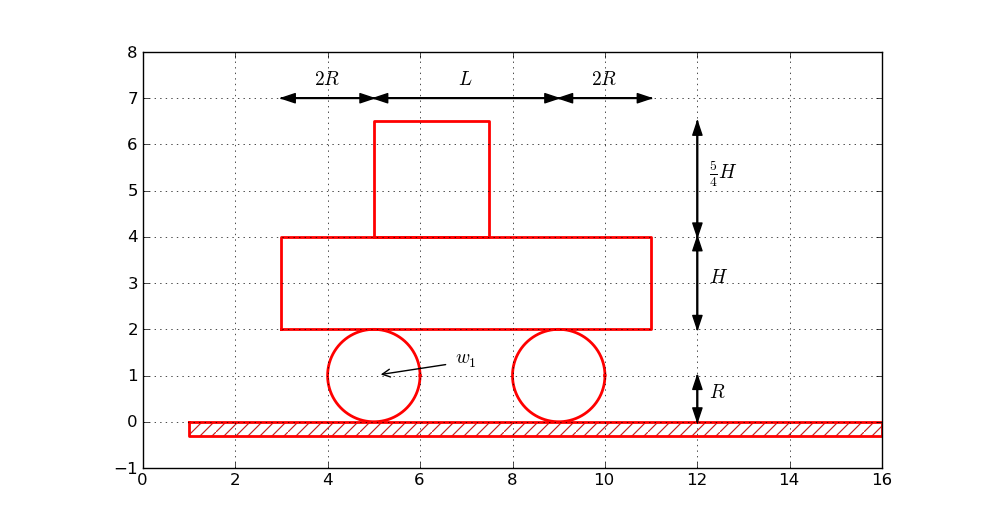
Sketch of a simple figure

Basic Drawing

A typical program creating these five elements is shown next. After importing the pysketcher package, the first task is always to define a coordinate system. Some graphics operations are done with a helper object called drawing_tool (imported from pysketcher). With the drawing area in place we can make the first Circle object in an intuitive fashion:

from pysketcher import *

R = 1    # radius of wheel
L = 4    # distance between wheels
H = 2    # height of vehicle body
w_1 = 5  # position of front wheel
drawing_tool.set_coordinate_system(xmin=0, xmax=w_1 + 2*L + 3*R,
                                   ymin=-1, ymax=2*R + 3*H)

wheel1 = Circle(center=(w_1, R), radius=R)

By using symbols for characteristic lengths in the drawing, rather than absolute lengths, it is easier to change dimensions later.

To translate the geometric information about the wheel1 object to instructions for the plotting engine (in this case Matplotlib), one calls the wheel1.draw(). To display all drawn objects, one issues drawing_tool.display(). The typical steps are hence:

wheel1 = Circle(center=(w_1, R), radius=R)
wheel1.draw()

# Define other objects and call their draw() methods
drawing_tool.display()
drawing_tool.savefig('tmp.png')  # store picture

The next wheel can be made by taking a copy of wheel1 and translating the object a distance (to the right) described by the vector \((4,0)\):

wheel2 = wheel1.copy()
wheel2.translate((L,0))

The two rectangles are made in an intuitive way:

under = Rectangle(lower_left_corner=(w_1-2*R, 2*R),
                  width=2*R + L + 2*R, height=H)
over  = Rectangle(lower_left_corner=(w_1, 2*R + H),
                  width=2.5*R, height=1.25*H)

Groups of Objects

Instead of calling the draw method of every object, we can group objects and call draw, or perform other operations, for the whole group. For example, we may collect the two wheels in a wheels group and the over and under rectangles in a body group. The whole vehicle is a composition of its wheels and body groups. The codes goes like

wheels  = Composition({'wheel1': wheel1, 'wheel2': wheel2})
body    = Composition({'under': under, 'over': over})

vehicle = Composition({'wheels': wheels, 'body': body})

The ground is illustrated by an object of type Wall, mostly used to indicate walls in sketches of mechanical systems. A Wall takes the x and y coordinates of some curve, and a thickness parameter, and creates a “thick” curve filled with a simple pattern. In this case the curve is just a flat line so the construction is made of two points on the ground line (\((w_1-L,0)\) and \((w_1+3L,0)\)):

ground = Wall(x=[w_1 - L, w_1 + 3*L], y=[0, 0], thickness=-0.3*R)

The negative thickness makes the pattern-filled rectangle appear below the defined line, otherwise it appears above.

We may now collect all the objects in a “top” object that contains the whole figure:

fig = Composition({'vehicle': vehicle, 'ground': ground})
fig.draw()  # send all figures to plotting backend
drawing_tool.display()
drawing_tool.savefig('tmp.png')

The fig.draw() call will visit all subgroups, their subgroups, and so in the hierarchical tree structure that we have collected, and call draw for every object.

Changing Line Styles and Colors

Controlling the line style, line color, and line width is fundamental when designing figures. The pysketcher package allows the user to control such properties in single objects, but also set global properties that are used if the object has no particular specification of the properties. Setting the global properties are done like

drawing_tool.set_linestyle('dashed')
drawing_tool.set_linecolor('black')
drawing_tool.set_linewidth(4)

At the object level the properties are specified in a similar way:

wheel1.set_linestyle('solid')
wheel1.set_linecolor('red')

and so on.

Geometric figures can be specified as filled, either with a color or with a special visual pattern:

# Set filling of all curves
drawing_tool.set_filled_curves(color='blue', pattern='/')

# Turn off filling of all curves
drawing_tool.set_filled_curves(False)

# Fill the wheel with red color
wheel1.set_filled_curves('red')

The Figure Composition as an Object Hierarchy

The composition of objects is hierarchical, as in a family, where each object has a parent and a number of children. Do a print fig to display the relations:

ground
    wall
vehicle
    body
        over
            rectangle
        under
            rectangle
    wheels
        wheel1
            arc
        wheel2
            arc

The indentation reflects how deep down in the hierarchy (family) we are. This output is to be interpreted as follows:

• fig contains two objects, ground and vehicle
• ground contains an object wall
• vehicle contains two objects, body and wheels
• body contains two objects, over and under
• wheels contains two objects, wheel1 and wheel2

More detailed information can be printed by

print fig.show_hierarchy('std')

yielding the output

ground (Wall):
    wall (Curve): 4 coords fillcolor='white' fillpattern='/'
vehicle (Composition):
    body (Composition):
        over (Rectangle):
            rectangle (Curve): 5 coords
        under (Rectangle):
            rectangle (Curve): 5 coords
    wheels (Composition):
        wheel1 (Circle):
            arc (Curve): 181 coords
        wheel2 (Circle):
            arc (Curve): 181 coords

Here we can see the class type for each figure object, how many coordinates that are involved in basic figures (Curve objects), and special settings of the basic figure (fillcolor, line types, etc.). For example, wheel2 is a Circle object consisting of an arc, which is a Curve object consisting of 181 coordinates (the points needed to draw a smooth circle). The Curve objects are the only objects that really holds specific coordinates to be drawn. The other object types are just compositions used to group parts of the complete figure.

One can also get a graphical overview of the hierarchy of figure objects that build up a particular figure fig. Just call fig.graphviz_dot('fig') to produce a file fig.dot in the dot format. This file contains relations between parent and child objects in the figure and can be turned into an image, as in Figure Hierarchical relation between figure objects, by running the dot program:

Terminal> dot -Tpng -o fig.png fig.dot

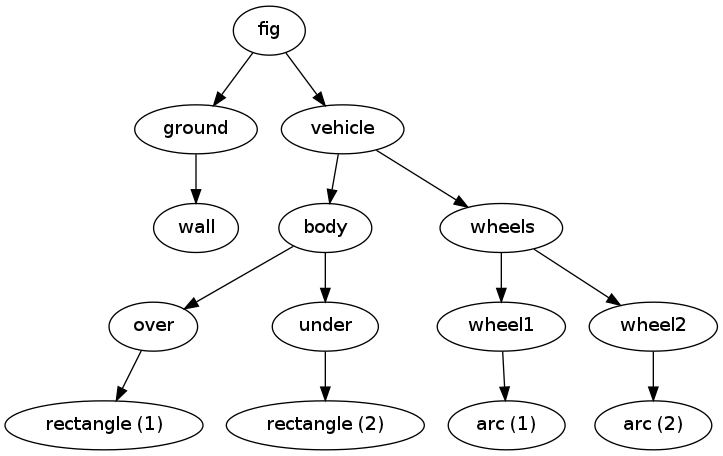
Hierarchical relation between figure objects

The call fig.graphviz_dot('fig', classname=True) makes a fig.dot file where the class type of each object is also visible, see Figure sketcher:fig:vehicle0:hier2. The ability to write out the object hierarchy or view it graphically can be of great help when working with complex figures that involve layers of subfigures.

Hierarchical relation between figure objects, including their class names

Any of the objects can in the program be reached through their names, e.g.,

fig['vehicle']
fig['vehicle']['wheels']
fig['vehicle']['wheels']['wheel2']
fig['vehicle']['wheels']['wheel2']['arc']
fig['vehicle']['wheels']['wheel2']['arc'].x  # x coords
fig['vehicle']['wheels']['wheel2']['arc'].y  # y coords
fig['vehicle']['wheels']['wheel2']['arc'].linestyle
fig['vehicle']['wheels']['wheel2']['arc'].linetype

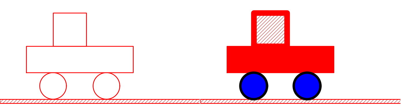
Grabbing a part of the figure this way is very handy for changing properties of that part, for example, colors, line styles (see Figure Left: Basic line-based drawing. Right: Thicker lines and filled parts):

fig['vehicle']['wheels'].set_filled_curves('blue')
fig['vehicle']['wheels'].set_linewidth(6)
fig['vehicle']['wheels'].set_linecolor('black')

fig['vehicle']['body']['under'].set_filled_curves('red')

fig['vehicle']['body']['over'].set_filled_curves(pattern='/')
fig['vehicle']['body']['over'].set_linewidth(14)
fig['vehicle']['body']['over']['rectangle'].linewidth = 4

The last line accesses the Curve object directly, while the line above, accesses the Rectangle object which will then set the linewidth of its Curve object, and other objects if it had any. The result of the actions above is shown in Figure Left: Basic line-based drawing. Right: Thicker lines and filled parts.

Left: Basic line-based drawing. Right: Thicker lines and filled parts

We can also change position of parts of the figure and thereby make animations, as shown next.

Animation: Translating the Vehicle

Can we make our little vehicle roll? A first attempt will be to fake rolling by just displacing all parts of the vehicle. The relevant parts constitute the fig['vehicle'] object. This part of the figure can be translated, rotated, and scaled. A translation along the ground means a translation in \(x\) direction, say a length \(L\) to the right:

fig['vehicle'].translate((L,0))

You need to erase, draw, and display to see the movement:

drawing_tool.erase()
fig.draw()
drawing_tool.display()

Without erasing the old position of the vehicle will remain in the figure so you get two vehicles. Without fig.draw() the new coordinates of the vehicle will not be communicated to the drawing tool, and without calling display the updated drawing will not be visible.

Let us make a velocity function and move the object according to that velocity in small steps of time:

def v(t):
    return -8*R*t*(1 - t/(2*R))

animate(fig, tp, action)

For small time steps dt the corresponding displacement is well approximated by dt*v(t) (we could integrate the velocity to obtain the exact position, but we would anyway need to calculate the displacement from time step to time step). The animate function takes as arguments some figure fig, a set of time points tp, and a user function action, and then a new figure is drawn for each time point and the user can through the provided action function modify desired parts of the figure. Here the action function will move the vehicle:

def move_vehicle(t, fig):
    x_displacement = dt*v(t)
    fig['vehicle'].translate((x_displacement, 0))

Defining a set of time points for the frames in the animation and performing the animation is done by

import numpy
tp = numpy.linspace(0, 2*R, 25)
dt = tp[1] - tp[0]  # time step

animate(fig, tp, move_vehicle, pause_per_frame=0.2)

The pause_per_frame adds a pause, here 0.2 seconds, between each frame.

We can also make a movie file of the animation:

files = animate(fig, tp, move_vehicle, moviefiles=True,
                pause_per_frame=0.2)

The files variable holds a string with the family of files constituting the frames in the movie, here 'tmp_frame*.png'. Making a movie out of the individual frames can be done in many ways. A simple approach is to make an animated GIF file with help of convert, a program in the ImageMagick software suite:

Terminal> convert -delay 20 tmp_frame*.png anim.gif
Terminal> animate anim.gif  # play movie

The delay between frames governs the speed of the movie. The anim.gif file can be embedded in a web page and shown as a movie the page is loaded into a web browser (just insert <img src="anim.gif"> in the HTML code to play the GIF animation).

The tool ffmpeg can alternatively be used, e.g.,

Terminal> ffmpeg -i "tmp_frame_%04d.png" -b 800k -r 25 \
          -vcodec mpeg4 -y -qmin 2 -qmax 31 anim.mpeg

An easy-to-use interface to movie-making tools is provided by the SciTools package:

from scitools.std import movie

# HTML page showing individual frames
movie(files, encoder='html', output_file='anim.html')

# Standard GIF file
movie(files, encoder='convert', output_file='anim.gif')

# AVI format
movie('tmp_*.png', encoder='ffmpeg', fps=4,
      output_file='anim.avi') # requires ffmpeg package

# MPEG format
movie('tmp_*.png', encoder='ffmpeg', fps=4,
      output_file='anim2.mpeg', vodec='mpeg2video')
# or
movie(files, encoder='ppmtompeg', fps=24,
      output_file='anim.mpeg')  # requires the netpbm package

When difficulties with encoders and players arise, the simple web page for showing a movie, here anim.html (generated by the first movie command above), is a safe method that you always can rely on. You can try loading anim.html into a web browser, after first having run the present example in the file ``vehicle0.py` <http://hplgit.github.com/pysketcher/doc/src/sketcher/src-sketcher/vehicle0.py>`_. Alternatively, you can view a ready-made movie.

Animation: Rolling the Wheels

It is time to show rolling wheels. To this end, we make somewhat more complicated wheels with spokes as on a bicyle, formed by two crossing lines, see Figure Wheels with spokes to show rotation. The construction of the wheels will now involve a circle and two lines:

wheel1 = Composition({
    'wheel': Circle(center=(w_1, R), radius=R),
    'cross': Composition({'cross1': Line((w_1,0),   (w_1,2*R)),
                          'cross2': Line((w_1-R,R), (w_1+R,R))})})
wheel2 = wheel1.copy()
wheel2.translate((L,0))

Observe that wheel1.copy() copies all the objects that make up the first wheel, and wheel2.translate translates all the copied objects.

Wheels with spokes to show rotation

The move_vehicle function now needs to displace all the objects in the entire vehicle and also rotate the cross1 and cross2 objects in both wheels. The rotation angle follows from the fact that the arc length of a rolling wheel equals the displacement of the center of the wheel, leading to a rotation angle

angle = - x_displacement/R

With w_1 tracking the \(x\) coordinate of the center of the front wheel, we can rotate that wheel by

w1 = fig['vehicle']['wheels']['wheel1']
from math import degrees
w1.rotate(degrees(angle), center=(w_1, R))

The rotate function takes two parameters: the rotation angle (in degrees) and the center point of the rotation, which is the center of the wheel in this case. The other wheel is rotated by

w2 = fig['vehicle']['wheels']['wheel2']
w2.rotate(degrees(angle), center=(w_1 + L, R))

That is, the angle is the same, but the rotation point is different. The update of the center point is done by w_1 += displacement[0]. The complete move_vehicle function then becomes

w_1 = w_1 + L   # start position

def move_vehicle(t, fig):
    x_displacement = dt*v(t)
    fig['vehicle'].translate((x_displacement, 0))

    # Rotate wheels
    global w_1
    w_1 += x_displacement
    # R*angle = -x_displacement
    angle = - x_displacement/R
    w1 = fig['vehicle']['wheels']['wheel1']
    w1.rotate(degrees(angle), center=(w_1, R))
    w2 = fig['vehicle']['wheels']['wheel2']
    w2.rotate(degrees(angle), center=(w_1 + L, R))

The complete example is found in the file ``vehicle1.py` <http://hplgit.github.com/pysketcher/doc/src/sketcher/src-sketcher/vehicle1.py>`_. You may run this file or watch a ready-made movie.

The advantages with making figures this way through programming, rather than using interactive drawing programs, are numerous. For example, the objects are parameterized by variables so that various dimensions can easily be changed. Subparts of the figure, possible involving a lot of figure objects, can change color, linetype, filling or other properties through a single function call. Subparts of the figure can be rotated, translated, or scaled. Subparts of the figure can also be copied and moved to other parts of the drawing area. However, the single most important feature is probably the ability to make animations governed by mathematical formulas or data coming from physics simulations of the problem sketched in the drawing, as very simplistically shown in the example above.

Inner Workings of the Pysketcher Tool

We shall now explain how we can, quite easily, realize software with the capabilities demonstrated in the previous examples. Each object in the figure is represented as a class in a class hierarchy. Using inheritance, classes can inherit properties from parent classes and add new geometric features.

Class programming is a key technology for realizing Pysketcher. As soon as some classes are established, more are easily added. Enhanced functionality for all the classes is also easy to implement in common, generic code that can immediately be shared by all present and future classes. The fundamental data structure involved in the pysketcher package is a hierarchical tree, and much of the material on implementation issues targets how to traverse tree structures with recursive function calls in object hierarchies. This topic is of key relevance in a wide range of other applications as well. In total, the inner workings of Pysketcher constitute an excellent example on the power of class programming.

Example of Classes for Geometric Objects

We introduce class Shape as superclass for all specialized objects in a figure. This class does not store any data, but provides a series of functions that add functionality to all the subclasses. This will be shown later.

Simple Geometric Objects

One simple subclass is Rectangle:

class Rectangle(Shape):
    def __init__(self, lower_left_corner, width, height):
        p = lower_left_corner  # short form
        x = [p[0], p[0] + width,
             p[0] + width, p[0], p[0]]
        y = [p[1], p[1], p[1] + height,
             p[1] + height, p[1]]
        self.shapes = {'rectangle': Curve(x,y)}

Any subclass of Shape will have a constructor which takes geometric information about the shape of the object and creates a dictionary self.shapes with the shape built of simpler shapes. The most fundamental shape is Curve, which is just a collection of \((x,y)\) coordinates in two arrays x and y. Drawing the Curve object is a matter of plotting y versus x.

The Rectangle class illustrates how the constructor takes information about the lower left corner, the width and the height, and creates coordinate arrays x and y consisting of the four corners, plus the first one repeated such that plotting x and y will form a closed four-sided rectangle. This construction procedure demands that the rectangle will always be aligned with the \(x\) and \(y\) axis. However, we may easily rotate the rectangle about any point once the object is constructed.

Class Line constitutes a similar example:

class Line(Shape):
    def __init__(self, start, end):
        x = [start[0], end[0]]
        y = [start[1], end[1]]
        self.shapes = {'line': Curve(x, y)}

Here we only need two points, the start and end point on the line. However, we may add some useful functionality, e.g., the ability to give an \(x\) coordinate and have the class calculate the corresponding \(y\) coordinate:

def __call__(self, x):
    """Given x, return y on the line."""
    x, y = self.shapes['line'].x, self.shapes['line'].y
    self.a = (y[1] - y[0])/(x[1] - x[0])
    self.b = y[0] - self.a*x[0]
    return self.a*x + self.b

Unfortunately, this is too simplistic because vertical lines cannot be handled (infinite self.a). The source code of Line therefore provides a more general solution at the cost of significantly longer code with more tests.

A circle gives us somewhat increased complexity. Again we represent the geometric object by a Curve object, but this time the Curve object needs to store a large number of points on the curve such that a plotting program produces a visually smooth curve. The points on the circle must be calculated manually in the constructor of class Circle. The formulas for points \((x,y)\) on a curve with radius \(R\) and center at \((x_0, y_0)\) are given by

\[\begin{split}x &= x_0 + R\cos (t),\\ y &= y_0 + R\sin (t),\end{split}\]

where \(t\in [0, 2\pi]\). A discrete set of \(t\) values in this interval gives the corresponding set of \((x,y)\) coordinates on the circle. The user must specify the resolution, i.e., the number of \(t\) values, or equivalently, points on the circle. The circle’s radius and center must of course also be specified.

We can write the Circle class as

class Circle(Shape):
    def __init__(self, center, radius, resolution=180):
        self.center, self.radius = center, radius
        self.resolution = resolution

        t = linspace(0, 2*pi, resolution+1)
        x0 = center[0];  y0 = center[1]
        R = radius
        x = x0 + R*cos(t)
        y = y0 + R*sin(t)
        self.shapes = {'circle': Curve(x, y)}

As in class Line we can offer the possibility to give an angle \(\theta\) (equivalent to \(t\) in the formulas above) and then get the corresponding \(x\) and \(y\) coordinates:

def __call__(self, theta):
    """Return (x, y) point corresponding to angle theta."""
    return self.center[0] + self.radius*cos(theta), \
           self.center[1] + self.radius*sin(theta)

There is one flaw with this method: it yields illegal values after a translation, scaling, or rotation of the circle.

A part of a circle, an arc, is a frequent geometric object when drawing mechanical systems. The arc is constructed much like a circle, but \(t\) runs in \([\theta_0, \theta_1]\). Giving \(\theta_1\) and \(\theta_2\) the slightly more descriptive names start_angle and arc_angle, the code looks like this:

class Arc(Shape):
    def __init__(self, center, radius,
                 start_angle, arc_angle,
                 resolution=180):
        self.center = center
        self.radius = radius
        self.start_angle = start_angle*pi/180  # radians
        self.arc_angle = arc_angle*pi/180
        self.resolution = resolution

        t = linspace(self.start_angle,
                     self.start_angle + self.arc_angle,
                     resolution+1)
        x0 = center[0];  y0 = center[1]
        R = radius
        x = x0 + R*cos(t)
        y = y0 + R*sin(t)
        self.shapes = {'arc': Curve(x, y)}

Having the Arc class, a Circle can alternatively befined as a subclass specializing the arc to a circle:

class Circle(Arc):
    def __init__(self, center, radius, resolution=180):
        Arc.__init__(self, center, radius, 0, 360, resolution)

A wall is about drawing a curve, displacing the curve vertically by some thickness, and then filling the space between the curves by some pattern. The input is the x and y coordinate arrays of the curve and a thickness parameter. The computed coordinates will be a polygon: going along the originally curve and then back again along the vertically displaced curve. The relevant code becomes

class CurveWall(Shape):
    def __init__(self, x, y, thickness):
        # User's curve
        x1 = asarray(x, float)
        y1 = asarray(y, float)
        # Displaced curve (according to thickness)
        x2 = x1
        y2 = y1 + thickness
        # Combine x1,y1 with x2,y2 reversed
        from numpy import concatenate
        x = concatenate((x1, x2[-1::-1]))
        y = concatenate((y1, y2[-1::-1]))
        wall = Curve(x, y)
        wall.set_filled_curves(color='white', pattern='/')
        self.shapes = {'wall': wall}

Class Curve

Class Curve sits on the coordinates to be drawn, but how is that done? The constructor just stores the coordinates, while a method draw sends the coordinates to the plotting program to make a graph. Or more precisely, to avoid a lot of (e.g.) Matplotlib-specific plotting commands we have created a small layer with a simple programming interface to plotting programs. This makes it straightforward to change from Matplotlib to another plotting program. The programming interface is represented by the drawing_tool object and has a few functions:

• plot_curve for sending a curve in terms of \(x\) and \(y\) coordinates to the plotting program,
• set_coordinate_system for specifying the graphics area,
• erase for deleting all elements of the graph,
• set_grid for turning on a grid (convenient while constructing the plot),
• set_instruction_file for creating a separate file with all plotting commands (Matplotlib commands in our case),
• a series of set_X functions where X is some property like linecolor, linestyle, linewidth, filled_curves.

This is basically all we need to communicate to a plotting program.

Any class in the Shape hierarchy inherits set_X functions for setting properties of curves. This information is propagated to all other shape objects that make up the figure. Class Curve stores the line properties together with the coordinates of its curve and propagates this information to the plotting program. When saying vehicle.set_linewidth(10), all objects that make up the vehicle object will get a set_linewidth(10) call, but only the Curve object at the end of the chain will actually store the information and send it to the plotting program.

A rough sketch of class Curve reads

class Curve(Shape):
    """General curve as a sequence of (x,y) coordintes."""
    def __init__(self, x, y):
        self.x = asarray(x, dtype=float)
        self.y = asarray(y, dtype=float)

        self.linestyle = None
        self.linewidth = None
        self.linecolor = None
        self.fillcolor = None
        self.fillpattern = None
        self.arrow = None

    def draw(self):
        drawing_tool.plot_curve(
            self.x, self.y,
            self.linestyle, self.linewidth, self.linecolor,
            self.arrow, self.fillcolor, self.fillpattern)

    def set_linewidth(self, width):
        self.linewidth = width

    det set_linestyle(self, style):
        self.linestyle = style
    ...

Compound Geometric Objects

The simple classes Line, Arc, and Circle could define the geometric shape through just one Curve object. More complicated figure elements are built from instances of various subclasses of Shape. Classes used for professional drawings soon get quite complex in composition and have a lot of geometric details, so here we prefer to make a very simple composition: the already drawn vehicle from Figure ref:ref:sketcher:fig:vehicle0. That is, instead of composing the drawing in a Python code we make a class Vehicle0 for doing the same thing, and derive it from Shape.

The Shape hierarchy is found in the pysketcher package, so to use these classes or derive a new one, we need to import pysketcher. The constructor of class Vehicle0 performs approximately the same statements as in the example program we developed for making the drawing in Figure ref:ref:sketcher:fig:vehicle0.

class Vehicle0(Shape):
    def __init__(self, w_1, R, L, H):
        wheel1 = Circle(center=(w_1, R), radius=R)
        wheel2 = wheel1.copy()
        wheel2.translate((L,0))

        under = Rectangle(lower_left_corner=(w_1-2*R, 2*R),
                          width=2*R + L + 2*R, height=H)
        over  = Rectangle(lower_left_corner=(w_1, 2*R + H),
                          width=2.5*R, height=1.25*H)

        wheels = Composition(
            {'wheel1': wheel1, 'wheel2': wheel2})
        body = Composition(
            {'under': under, 'over': over})

        vehicle = Composition({'wheels': wheels, 'body': body})
        xmax = w_1 + 2*L + 3*R
        ground = Wall(x=[R, xmax], y=[0, 0], thickness=-0.3*R)

        self.shapes = {'vehicle': vehicle, 'ground': ground}

Any subclass of Shape must define the shapes attribute, otherwise the inherited draw method (and a lot of other methods too) will not work.

The painting of the vehicle could be offered by a method:

def colorful(self):
    wheels = self.shapes['vehicle']['wheels']
    wheels.set_filled_curves('blue')
    wheels.set_linewidth(6)
    wheels.set_linecolor('black')
    under = self.shapes['vehicle']['body']['under']
    under.set_filled_curves('red')
    over = self.shapes['vehicle']['body']['over']
    over.set_filled_curves(pattern='/')
    over.set_linewidth(14)

The usage of the class is simple: after having set up an appropriate coordinate system a s previously shown, we can do

vehicle = Vehicle0(w_1, R, L, H)
vehicle.draw()
drawing_tool.display()

The color from Figure Left: Basic line-based drawing. Right: Thicker lines and filled parts is realized by

drawing_tool.erase()
vehicle.colorful()
vehicle.draw()
drawing_tool.display()

A complete code defining and using class Vehicle0 is found in the file ``vehicle2.py` <http://hplgit.github.com/pysketcher/doc/src/sketcher/src-sketcher/vehicle2.py>`_.

The pysketcher package contains a wide range of classes for various geometrical objects, particularly those that are frequently used in drawings of mechanical systems.

Adding Functionality via Recursion

The really powerful feature of our class hierarchy is that we can add much functionality to the superclass Shape and to the “bottom” classes Curve, and all other classes for all types of geometrical shapes immediately get the new functionality. To explain the idea we first have to look at the draw method, which all classes in the Shape hierarchy must have. The inner workings of the draw method explain the secrets of how a series of other useful operations on figures can be implemented.

We work with two types of class hierarchies: one Python class hierarchy, with Shape as superclass, and one object hierarchy of figure elements in a specific figure. A subclass of Shape stores its figure in the self.shapes dictionary. This dictionary represents the object hierarchy of figure elements for that class. We want to make one draw call for an instance, say our class Vehicle0, and then we want this call to be propagated to all objects that are contained in self.shapes and all is nested subdictionaries. How is this done?

The natural starting point is to call draw for each Shape object in the self.shapes dictionary:

def draw(self):
    for shape in self.shapes:
        self.shapes[shape].draw()

This general method can be provided by class Shape and inherited in subclasses like Vehicle0. Let v be a Vehicle0 instance. Seemingly, a call v.draw() just calls

v.shapes['vehicle'].draw()
v.shapes['ground'].draw()

However, in the former call we call the draw method of a Composition object whose self.shapes attributed has two elements: wheels and body. Since class Composition inherits the same draw method, this method will run through self.shapes and call wheels.draw() and body.draw(). Now, the wheels object is also a Composition with the same draw method, which will run through the shapes dictionary, now containing the wheel1 and and wheel2 objects. The wheel1 object is a Circle, so calling wheel1.draw() calls the draw method in class Circle, but this is the same draw method as shown above. This method will therefore traverse the circle’s shapes dictionary, which we have seen consists of one Curve element.

The Curve object holds the coordinates to be plotted so here draw really needs to do something “physical”, namely send the coordinates to the plotting program. The draw method is outlined in the short listing of class Curve shown previously.

We can go to any of the other shape objects that appear in the figure hierarchy and follow their draw calls in the similar way. Every time, a draw call will invoke a new draw call, until we eventually hit a Curve object in the “botton” of the figure hierarchy, and then that part of the figure is really plotted (or more precisely, the coordinates are sent to a plotting program).

When a method calls itself, such as draw does, the calls are known as recursive and the programming principle is referred to as recursion. This technique is very often used to traverse hierarchical structures like the figure structures we work with here. Even though the hierarchy of objects building up a figure are of different types, they all inherit the same draw method and therefore exhibit the same behavior with respect to drawing. Only the Curve object has a different draw method, which does not lead to more recursion. Without this different draw method in class Curve, the repeated draw calls would go on forever.

Understanding recursion is usually a challenge. To get a better idea of how recursion works, we have equipped class Shape with a method recurse which just visits all the objects in the shapes dictionary and prints out a message for each object. This feature allows us to trace the execution and see exactly where we are in the hierarchy and which objects that are visited.

The recurse method is very similar to draw:

def recurse(self, name, indent=0):
    # print message where we are (name is where we come from)
    for shape in self.shapes:
        # print message about which object to visit
        self.shapes[shape].recurse(indent+2, shape)

The indent parameter governs how much the message from this recurse method is intended. We increase indent by 2 for every level in the hierarchy. This makes it easy to see on the printout how far down in the hierarchy we are.

A typical message written by recurse when name is body and the shapes dictionary contains two entries, over and under, will be

Composition: body.shapes has entries 'over', 'under'
call body.shapes["over"].recurse("over", 6)

The number of leading blanks on each line corresponds to the value of indent. The code printing out such messages looks like

def recurse(self, name, indent=0):
    space = ' '*indent
    print space, '%s: %s.shapes has entries' % \
          (self.__class__.__name__, name), \
          str(list(self.shapes.keys()))[1:-1]

    for shape in self.shapes:
        print space,
        print 'call %s.shapes["%s"].recurse("%s", %d)' % \
              (name, shape, shape, indent+2)
        self.shapes[shape].recurse(shape, indent+2)

Let us follow a v.recurse('vehicle') call in detail, v being a Vehicle0 instance. Before looking into the output from recurse, let us get an overview of the figure hierarchy in the v object (as produced by print v)

ground
    wall
vehicle
    body
        over
            rectangle
        under
            rectangle
    wheels
        wheel1
            arc
        wheel2
            arc

The recurse method performs the same kind of traversal of the hierarchy, but writes out and explains a lot more.

The data structure represented by v.shapes is known as a tree. As in physical trees, there is a root, here the v.shapes dictionary. A graphical illustration of the tree (upside down) is shown in Figure sketcher:fig:Vehicle0:hier2. From the root there are one or more branches, here two: ground and vehicle. Following the vehicle branch, it has two new branches, body and wheels. Relationships as in family trees are often used to describe the relations in object trees too: we say that vehicle is the parent of body and that body is a child of vehicle. The term node is also often used to describe an element in a tree. A node may have several other nodes as descendants.

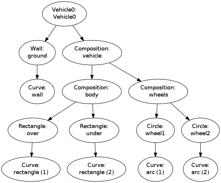
Hierarchy of figure elements in an instance of class `Vehicle0`

Recursion is the principal programming technique to traverse tree structures. Any object in the tree can be viewed as a root of a subtree. For example, wheels is the root of a subtree that branches into wheel1 and wheel2. So when processing an object in the tree, we imagine we process the root and then recurse into a subtree, but the first object we recurse into can be viewed as the root of the subtree, so the processing procedure of the parent object can be repeated.

A recommended next step is to simulate the recurse method by hand and carefully check that what happens in the visits to recurse is consistent with the output listed below. Although tedious, this is a major exercise that guaranteed will help to demystify recursion. Also remember that it requires some efforts to understand recursion.

A part of the printout of v.recurse('vehicle') looks like

 Vehicle0: vehicle.shapes has entries 'ground', 'vehicle'
 call vehicle.shapes["ground"].recurse("ground", 2)
   Wall: ground.shapes has entries 'wall'
   call ground.shapes["wall"].recurse("wall", 4)
     reached "bottom" object Curve
 call vehicle.shapes["vehicle"].recurse("vehicle", 2)
   Composition: vehicle.shapes has entries 'body', 'wheels'
   call vehicle.shapes["body"].recurse("body", 4)
     Composition: body.shapes has entries 'over', 'under'
     call body.shapes["over"].recurse("over", 6)
       Rectangle: over.shapes has entries 'rectangle'
       call over.shapes["rectangle"].recurse("rectangle", 8)
         reached "bottom" object Curve
     call body.shapes["under"].recurse("under", 6)
       Rectangle: under.shapes has entries 'rectangle'
       call under.shapes["rectangle"].recurse("rectangle", 8)
         reached "bottom" object Curve
...

This example should clearly demonstrate the principle that we can start at any object in the tree and do a recursive set of calls with that object as root.

Scaling, Translating, and Rotating a Figure

With recursion, as explained in the previous section, we can within minutes equip all classes in the Shape hierarchy, both present and future ones, with the ability to scale the figure, translate it, or rotate it. This added functionality requires only a few lines of code.

Scaling

We start with the simplest of the three geometric transformations, namely scaling. For a Curve instance containing a set of \(n\) coordinates \((x_i,y_i)\) that make up a curve, scaling by a factor \(a\) means that we multiply all the \(x\) and \(y\) coordinates by \(a\):

\[x_i \leftarrow ax_i,\quad y_i\leftarrow ay_i, \quad i=0,\ldots,n-1\thinspace .\]

Here we apply the arrow as an assignment operator. The corresponding Python implementation in class Curve reads

class Curve:
    ...
    def scale(self, factor):
        self.x = factor*self.x
        self.y = factor*self.y

Note here that self.x and self.y are Numerical Python arrays, so that multiplication by a scalar number factor is a vectorized operation.

An even more efficient implementation is to make use of in-place multiplication in the arrays, as this saves the creation of temporary arrays like factor*self.x, which is then assigned to self.x:

class Curve:
    ...
    def scale(self, factor):
        self.x *= factor
        self.y *= factor

In an instance of a subclass of Shape, the meaning of a method scale is to run through all objects in the dictionary shapes and ask each object to scale itself. This is the same delegation of actions to subclass instances as we do in the draw (or recurse) method. All all objects, except Curve instances, can share the same implementation of the scale method. Therefore, we place the scale method in the superclass Shape such that all subclasses inherit the method. Since scale and draw are so similar, we can easily implement the scale method in class Shape by copying and editing the draw method:

class Shape:
    ...
    def scale(self, factor):
        for shape in self.shapes:
            self.shapes[shape].scale(factor)

This is all we have to do in order to equip all subclasses of Shape with scaling functionality! Any piece of the figure will scale itself, in the same manner as it can draw itself.

Translation

A set of coordinates \((x_i, y_i)\) can be translated \(v_0\) units in the \(x\) direction and \(v_1\) units in the \(y\) direction using the formulas

\[x_i\leftarrow x_i+v_0,\quad y_i\leftarrow y_i+v_1,\quad i=0,\ldots,n-1\thinspace .\]

The natural specification of the translation is in terms of a vector \(v=(v_0,v_1)\). The corresponding Python implementation in class Curve becomes

class Curve:
    ...
    def translate(self, v):
        self.x += v[0]
        self.y += v[1]

The translation operation for a shape object is very similar to the scaling and drawing operations. This means that we can implement a common method translate in the superclass Shape. The code is parallel to the scale method:

class Shape:
    ....
    def translate(self, v):
        for shape in self.shapes:
            self.shapes[shape].translate(v)

Rotation

Rotating a figure is more complicated than scaling and translating. A counter clockwise rotation of \(\theta\) degrees for a set of coordinates \((x_i,y_i)\) is given by

\[\begin{split}\bar x_i &\leftarrow x_i\cos\theta - y_i\sin\theta,\\ \bar y_i &\leftarrow x_i\sin\theta + y_i\cos\theta\thinspace .\end{split}\]

This rotation is performed around the origin. If we want the figure to be rotated with respect to a general point \((x,y)\), we need to extend the formulas above:

\[\begin{split}\bar x_i &\leftarrow x + (x_i -x)\cos\theta - (y_i -y)\sin\theta,\\ \bar y_i &\leftarrow y + (x_i -x)\sin\theta + (y_i -y)\cos\theta\thinspace .\end{split}\]

The Python implementation in class Curve, assuming that \(\theta\) is given in degrees and not in radians, becomes

def rotate(self, angle, center):
    angle = radians(angle)
    x, y = center
    c = cos(angle);  s = sin(angle)
    xnew = x + (self.x - x)*c - (self.y - y)*s
    ynew = y + (self.x - x)*s + (self.y - y)*c
    self.x = xnew
    self.y = ynew

The rotate method in class Shape is identical to the draw, scale, and translate methods except that we recurse into self.rotate(angle, center).

We have already seen the rotate method in action when animating the rolling wheel at the end of the section Animation: Rolling the Wheels.